In this article, I am going to show you how to choose the number of principal components when using principal component analysis for dimensionality reduction.

In the first section, I am going to give you a short answer for those of you who are in a hurry and want to get something working. Later, I am going to provide a more extended explanation for those of you who are interested in understanding PCA.

Short answer

Don’t do it. Don’t choose the number of components manually. Instead of that, use the option that allows you to set the variance of the input that is supposed to be explained by the generated components.

Remember to scale the data to the range between 0 and 1 before using PCA!

from sklearn.preprocessing import MinMaxScaler
scaler = MinMaxScaler()
data_rescaled = scaler.fit_transform(data)

Typically, we want the explained variance to be between 95–99%. In Scikit-learn we can set it like this:

//95% of variance
from sklearn.decomposition import PCA
pca = PCA(n_components = 0.95)
pca.fit(data_rescaled)
reduced = pca.transform(data_rescaled)

//99% of variance
from sklearn.decomposition import PCA
pca = PCA(n_components = 0.99)
pca.fit(data_rescaled)
reduced = pca.transform(data_rescaled)

Long answer

How PCA works

First, the PCA algorithm is going to standardize the input data frame, calculate the covariance matrix of the features.

Now, let’s try to imagine that every value from the covariance matrix is a vector. That vector indicates a direction in the n-dimensional space (n is the number of features in the original data frame). What is a vector? We can imagine that as an “arrow” pointing in some direction in that n-dimensional space.

Those vectors can be “averaged” by generating another vector that “points” more or less in the same direction as all of those averaged vectors. We call it an eigenvector. It also has a value (let’s imagine it as a “length” of the “arrow”) that is correlated with the number of vectors averaged by the eigenvector (the more averaged covariance vectors, the larger the eigenvalue).

After that, we sort the eigenvectors by their eigenvalues. Remember that we have already chosen the cut off point (the desired variance that is supposed to be explained by the principal components). It means we can select the eigenvectors which add up to the desired threshold of explained variance.

Now, we multiply the standardized feature data frame by the matrix of principal components, and as a result, we get the compressed representation of the input data.

There is a great article written by Zakaria Jaadi, who explains PCA and shows step-by-step how to calculate the result.

How to select the number of components

Now, we know that the principal components explain a part of the variance. From the Scikit-learn implementation, we can get the information about the explained variance and plot the cumulative variance.

pca = PCA().fit(data_rescaled)

% matplotlib inline
import matplotlib.pyplot as plt
plt.rcParams["figure.figsize"] = (12,6)

fig, ax = plt.subplots()
xi = np.arange(1, 11, step=1)
y = np.cumsum(pca.explained_variance_ratio_)

plt.ylim(0.0,1.1)
plt.plot(xi, y, marker='o', linestyle='--', color='b')

plt.xlabel('Number of Components')
plt.xticks(np.arange(0, 11, step=1)) #change from 0-based array index to 1-based human-readable label
plt.ylabel('Cumulative variance (%)')
plt.title('The number of components needed to explain variance')

plt.axhline(y=0.95, color='r', linestyle='-')
plt.text(0.5, 0.85, '95% cut-off threshold', color = 'red', fontsize=16)

ax.grid(axis='x')
plt.show()

On the plotted chart, we see what number of principal components we need.

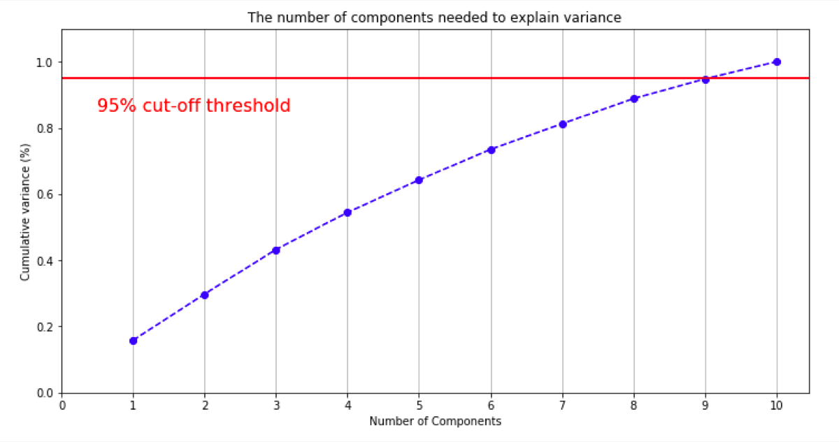
In this case, to get 95% of variance explained I need 9 principal components.

PCA — how to choose the number of components?

Short answer

Long answer

How PCA works

How to select the number of components

How to avoid bias against underrepresented target classes while training a machine learning model

Generalized Linear Models — Using linear regression when the dependent variable does not follow Gaussian distribution

PCA — how to choose the number of components?

Short answer

Long answer

How PCA works

How to select the number of components

How to avoid bias against underrepresented target classes while training a machine learning model

Generalized Linear Models — Using linear regression when the dependent variable does not follow Gaussian distribution

Related Posts

A.I. in production: your next stylist is going to be a neural network

What is the difference between training, validation, and test sets in machine learning

How to plot the decision trees from XGBoost classifier