F1 score is a classifier metric which calculates a mean of precision and recall in a way that emphasizes the lowest value.

If you want to understand how it works, keep reading ;)

How it works

F1 score is based on precision and recall. To show the F1 score behavior, I am going to generate real numbers between 0 and 1 and use them as an input of F1 score.

Later, I am going to draw a plot that hopefully will be helpful in understanding the F1 score.

import numpy as np
import pandas as pd
from mpl_toolkits.mplot3d import Axes3D
import matplotlib.gridspec as gridspec
import matplotlib.pyplot as plt

precision = np.arange(0, 1.01, 0.01)
recall = np.arange(0, 1.01, 0.01)

all_values = np.transpose([np.tile(precision, len(recall)), np.repeat(recall, len(precision))])
all_values = pd.DataFrame(all_values, columns=['precision', 'recall'])

The formula of F1 score looks like this:

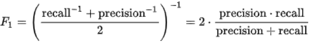
so I can use the following function to calculate the F1 score:

def f1_score(precision, recall):
    numerator = precision * recall
    denominator = precision + recall
    return 2 * numerator / denominator

all_values['f1_score'] = all_values.apply(lambda x: f1_score(x[0], x[1]), axis = 1)

Now I can plot a chart of the precision and recall (as x and y-axis) and their corresponding F1 score (as the z-axis).

def plot(precision, recall, f_score, f_score_label):
    plt.rcParams["figure.figsize"] = (20,10)

    fig = plt.figure()
    gs = gridspec.GridSpec(1, 2)

    ax = plt.subplot(gs[0, 0], projection='3d')
    ax.plot_trisurf(precision, recall, f_score, cmap=plt.cm.jet, linewidth=0.2, vmin = 0, vmax = 1)
    ax.set_xlabel('precision')
    ax.set_ylabel('recall')
    ax.set_zlabel(f_score_label, rotation = 0)
    ax.view_init(30, -125)

    ax2 = plt.subplot(gs[0, 1])
    sc = ax2.scatter(precision, recall, c = f_score, cmap=plt.cm.jet, vmin = 0, vmax = 1)

    ax2.set_xlabel('precision')
    ax2.set_ylabel('recall')

    plt.colorbar(sc)

    plt.show()

plot(all_values['precision'], all_values['recall'], all_values['f1_score'], f_score_label = 'F1 score')

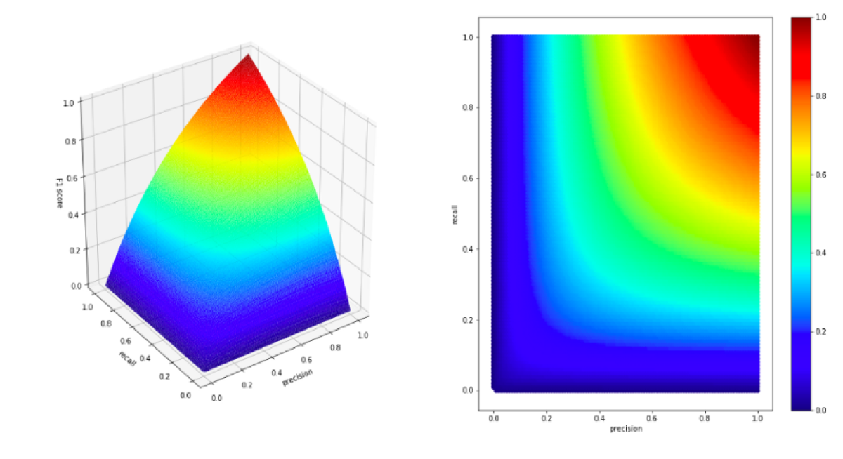
What do we see on the chart?

Let’s begin by looking at extreme values.
For example precision = 1 and recall = 0. It looks that in this case precision is ignored, and the F1 score remain equal to 0.
It behaves like that in all cases. If one of the parameters is small, the second one no longer matters.

As I mentioned at the beginning, F1 score emphasizes the lowest value.

Harmonic mean

Why does it behave like that? The F1 score is based on the harmonic mean.

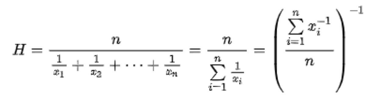
The harmonic mean is defined as the reciprocal of the arithmetic mean of the reciprocals. Because of that, the result is not sensitive to extremely large values.

On the other hand, not all outliers are ignored. Extremely low values have a significant influence on the result.

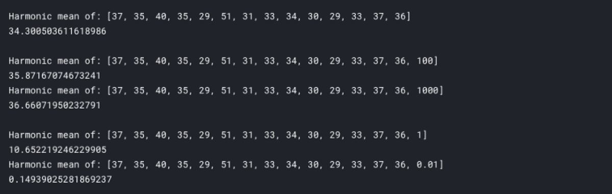
Let’s look at examples harmonic mean:

from scipy import stats

print('Harmonic mean of: ' + str([37, 35, 40, 35, 29, 51, 31, 33, 34, 30, 29, 33, 37, 36]))
print(stats.hmean([37, 35, 40, 35, 29, 51, 31, 33, 34, 30, 29, 33, 37, 36]))
print()

print('Harmonic mean of: ' + str([37, 35, 40, 35, 29, 51, 31, 33, 34, 30, 29, 33, 37, 36, 100]))
print(stats.hmean([37, 35, 40, 35, 29, 51, 31, 33, 34, 30, 29, 33, 37, 36, 100])) #added one large value
print('Harmonic mean of: ' + str([37, 35, 40, 35, 29, 51, 31, 33, 34, 30, 29, 33, 37, 36, 1000]))
print(stats.hmean([37, 35, 40, 35, 29, 51, 31, 33, 34, 30, 29, 33, 37, 36, 1000])) #added one extremely large value
print()

print('Harmonic mean of: ' + str([37, 35, 40, 35, 29, 51, 31, 33, 34, 30, 29, 33, 37, 36, 1]))
print(stats.hmean([37, 35, 40, 35, 29, 51, 31, 33, 34, 30, 29, 33, 37, 36, 1])) # added one small value
print('Harmonic mean of: ' + str([37, 35, 40, 35, 29, 51, 31, 33, 34, 30, 29, 33, 37, 36, 0.01]))
print(stats.hmean([37, 35, 40, 35, 29, 51, 31, 33, 34, 30, 29, 33, 37, 36, 0.01])) # added one extremely small value

Such a function is a perfect choice for the scoring metric of a classifier because useless classifiers get a meager score.

For example, if I created a fake “classifier” that tells a doctor whether a patient has the flu or not. My classifier ignores the input and always returns the same prediction: “has flu.” The recall of this classifier is going to be 1 because I correctly classified all sick patients as sick, but the precision is near 0 because of a considerable number of false positives.
If I use F1 score as a metric, that classifier is going to get a low score.

F1 score interpretation

Using F1 score as a metric, we are sure that if the F1 score is high, both precision and recall of the classifier indicate good results.

That characteristic of the metric allows us to compare the performance of two classifiers using just one metric and still be sure that the classifiers are not making some horrible mistakes that are unnoticed by the code which scores their output.

If we have a classifier which F1 score is low, we can’t tell whether it has problems with false positives or false negatives. In this case, the best way to “debug” such a classifier is to use confusion matrix to diagnose the problem and then look at the problematic cases in the validation or test dataset.

Fβ score

F1 score is just a special case of a more generic metric called Fβ score. This metric is also available in Scikit-learn: sklearn.metrics.fbeta_score

The formula of Fβ score is slightly different.

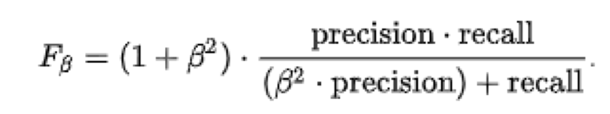
Because we multiply only one parameter of the denominator by β-squared, we can use β to make Fβ more sensitive to low values of either precision or recall. Yes, we can choose!

First, I am going to modify the implementation of my f1_score function and add “beta” parameter.

def fbeta_score(beta, precision, recall):
    numerator = precision * recall
    denominator = (beta**2 * precision) + recall
    return (1 + beta**2) * numerator / denominator

Let’s look at a chart of F2 score (Fβ with β = 2)

all_values['f2_score'] = all_values.apply(lambda x: fbeta_score(2, x[0], x[1]), axis = 1)

plot(all_values['precision'], all_values['recall'], all_values['f2_score'], f_score_label = 'F2 score')

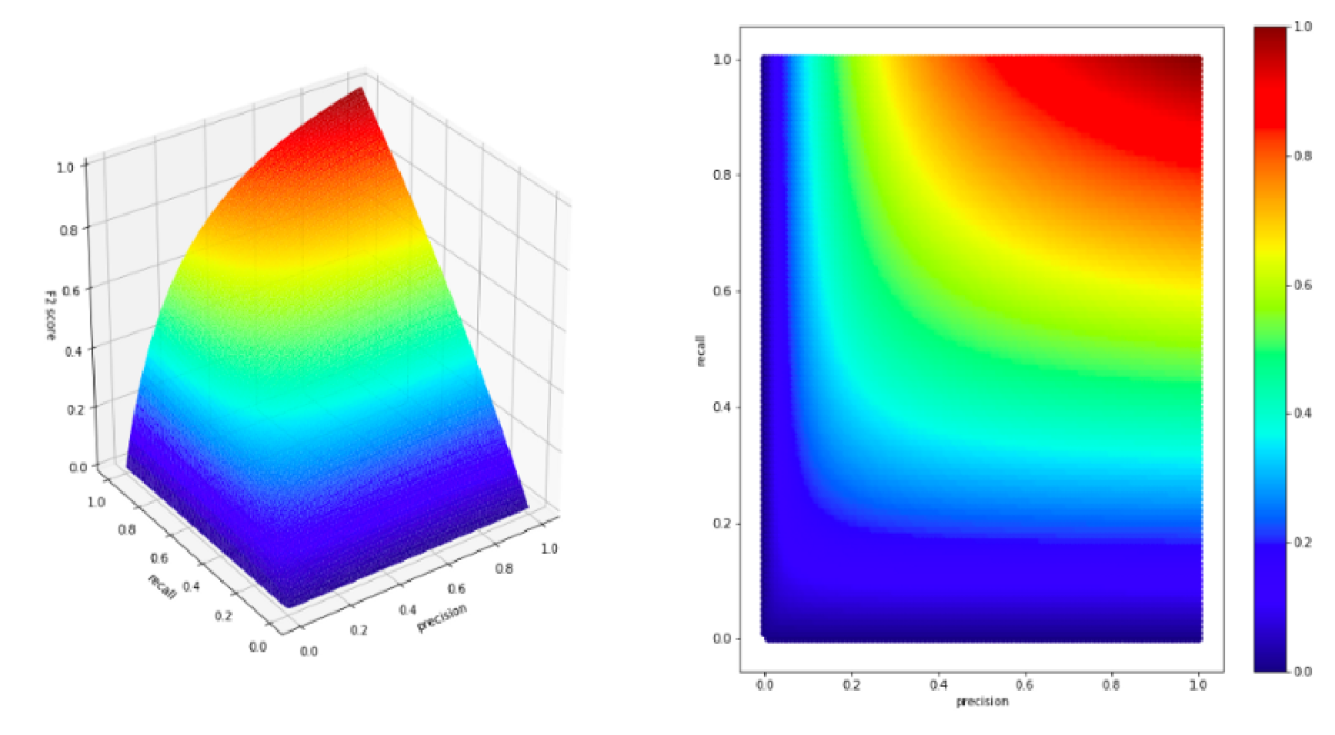
The first thing, we notice is the fact the values are skewed a little. Let’s look at the part where recall has value 0.2. In that case, the precision does not matter. The recall parameter dominates the F2 score. It means that in the case of F2 score, the recall has a higher weight than precision.

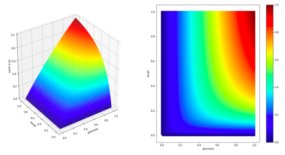
On the other hand, if we want to create a metric that is more sensitive to the value of the precision parameter, we must use a β value smaller than 1.

all_values['f05_score'] = all_values.apply(lambda x: fbeta_score(0.5, x[0], x[1]), axis = 1)

plot(all_values['precision'], all_values['recall'], all_values['f05_score'], f_score_label = 'F0.5 score')

When should we use Fβ score instead of F1 score?

In cases, when one of the metrics (precision or recall) is more important from the business perspective. It depends, how we are going to use the classifier and what kind of errors is more problematic.

In my previous blog post about classifier metrics, I used radar and detecting airplanes as an example in which both precision and recall can be used as a score.

If I used Fβ score, I could decide that recall is more important to me. After all, in my example, we will survive a false positive, but a false negative has grave consequences.

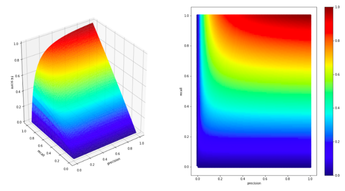
To make a scorer that punishes a classifier more for false negatives, I could set a higher β parameter and for example, use F4 score as a metric.

all_values['f4_score'] = all_values.apply(lambda x: fbeta_score(4, x[0], x[1]), axis = 1)

plot(all_values['precision'], all_values['recall'], all_values['f4_score'], f_score_label = 'F4 score')

F1 score explained

How it works

Harmonic mean

F1 score interpretation

Fβ score

When should we use Fβ score instead of F1 score?

How to display a progress bar in Jupyter Notebook

The optimal learning rate during fine-tuning of an artificial neural network

F1 score explained

How it works

Harmonic mean

F1 score interpretation

Fβ score

When should we use Fβ score instead of F1 score?

How to display a progress bar in Jupyter Notebook

The optimal learning rate during fine-tuning of an artificial neural network

Related Posts

I worked as a data scientist and that was the worst job I have ever had.

How to remove outliers from Seaborn boxplot charts

A.I. in production: your next stylist is going to be a neural network